Via research in the workplace, consultants, University and research center contacts and open source codes available in geophysics websites on the internet, CImaGeo develops its own programs for seismic data processing with the objective of better imaging and noise attenuation, offering a product of greater precision to our clients.
CImaGeo offers the following softwares for processing or process parameter calculation:
The software 1, 2, and 3 are used together for calculating Static Corrections for land seismic data.
1- Reflection Seismogram First Break Picking Software
The time determination of the first signals in each reflection seismogram (First Break “Picking”) is calculated through semiautomatic search algorithms for the times of these seismic traces.
The seismic data is limited in time and space to a window which contains the first signals that arrived from the geophones, permitting (or not) the application of a “Linear Move Out” (LMO) correction with representative velocity of the layer below the Weathering Zone. After a desired event in one of the traces of the domain (family) has been chosen (common PT, common Station, common Offset …) by the geophysicist, the program automatically searches, using one or more algorithms, through all the other traces and using rapid visual inspection, the geophysicist can validate (or not) that automatic determination:
i) If validated, the next family is offered on your screen, with the “picking” already occurring based on the previous result.
ii) If the geophysicist considers the automatic determination to be unsatisfactory, he can manually correct it and repeat the process for that family until the “picking” is considered to be of good quality.
When the quality of the first break is good, the arrival time of the “picking” events can occur in a rapid manner and with good precision. On the other hand, when the quality is poor, the difficulty to determine the arrival times is significant, requiring lots of practice and a great deal of effort by the processor.
First Break “Picking”
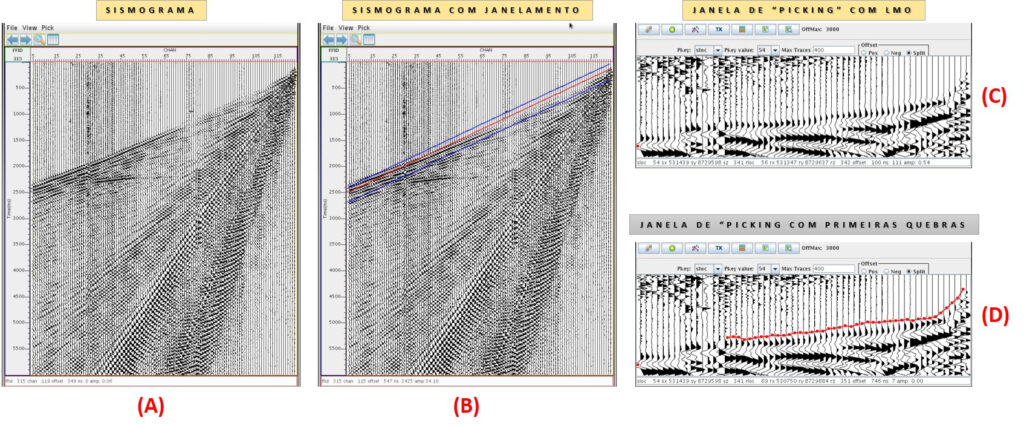
(A) Seismogram (B) Seismogram with windowing (C) ”Picking” window with LMO (D) “Picking” window with First Breaks. The figure above summarizes the “Picking” stages. Figure (A) shows a field seismogram with a six second length. Figure (B) shows the same seismogram with windowing that will be carried out to limit the data for the First Break “Picking”. Figure (C) is a “Picking” window and (D) is “Picking” carried out on the seismogram.
2- Interpretation Software for the First Breaks with Refraction equations.
Having the previous stage arrival times of the first breaks at hand, they are plotted on a Time X Distance curve and are interpreted using refraction equations.
Of these interpretations, the various layers that make up the Low Velocity Zone (LVZ), which is also known as the Weathering Zone or “Weathering Layer”, are calculated, thus obtaining the velocities and the thicknesses of the numerous layers and the non-weathered layer velocity immediately below the LVZ.
This LVZ model will be used as an initial model that, together with the first break times, the topography line, the acquisition geometry and the final Datum, shall be used for the complete inversion through the Refraction Tomography Principal, for the static corrections calculation which should be applied to the LVZ topography correction data, simulating an elevation on a horizontal-plane on the Datum level.
LOW VELOCITY ZONE INITIAL MODEL CALCULATION
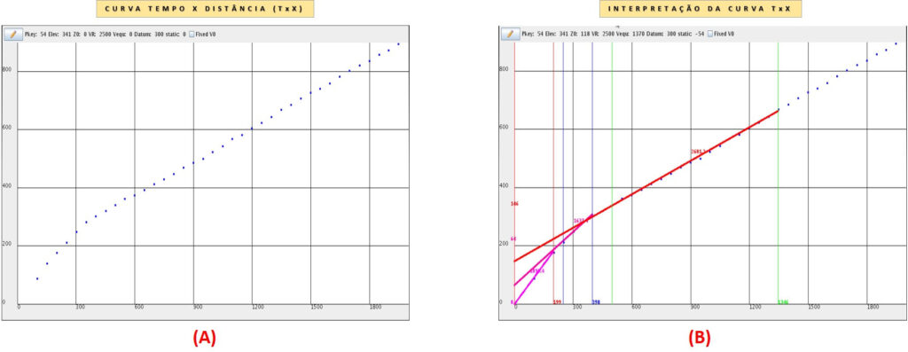
(A) Time X Distance Curve (TxX) (B) Curve Interpretation TxX. The figure above shows the Time X Distance graph construction of the first break times of shot 54. Part (A) of the figure, only the times versus the source-receptor distance is plotted. Part (B) of the figure presents an interpretation of the Time X Distance curve with the refraction equations. Note that part (B) describes the results of the interpretation at the top of the figure, with thickness values and LVZ layer velocities, which serve as an initial model for the tomographic inversion.
3- Seismic Refraction Tomography Software for the Static Correction Calculation in 2D and 3D Onshore Seismic Data.
The Seismic Refraction Tomography theory was developed as a doctorate thesis by the Geophysicist Wander Nogueira de Amorim in 1985 at the Federal University of Bahia (UFBA), under the guidance of Professor Dr. Peter Hubral.
The first break times of the reflection seismograms, determined in the first stage (software 11), together with the initial model calculated in the second stage (software 22), the topography and the geometric survey and Datum are organized mathematically to form an equation system of transit time of the refraction at the LVZ base.
Considering the initial model to be true, we model the first arrivals and compare the results of each synthetic time (ti,j) with its real respective “Picking” time, (ti,j). This error is used to modify the initial model, repeating the inversion process until the final error can be considered acceptable in the “Least Squares” sense:
Error = ǀ ti,j – ti,j ǀ = min
With the model duly set up, containing the thickness and velocity of the LVZ, the velocity of the non-weathered layer below the LVZ and the Datum, we can calculate the final static corrections for the application of the data. Once inverted with the complete time group of the first breaks, the final model can solve the short and long static problems, representing a high resolution, highly precise solution.
The figures below show the results obtained by seismic line processing with low precision static corrections and the same line processed with tomographic inversion static corrections.
INVERSION BY TOMOGRAPHY OF SEISMIC REFRACTION
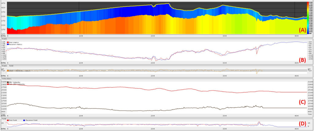
The figure above shows the final result of the tomographical inversion of the reflection seismogram first break times. Part (A) shows the topographic line, the LVZ (blue tones) and the sub-LVZ (in red and yellow tones), with the thickness scale on the left and the velocity scale on the right. Part (B) shows the shot static corrections (red) and the receptors (blue). Part (C) shows the velocities of the LVZ (black) and the sub-LVZ (red) and part (D) shows the redundancy of the shot static correction calculation (red) and the receptors (blue).
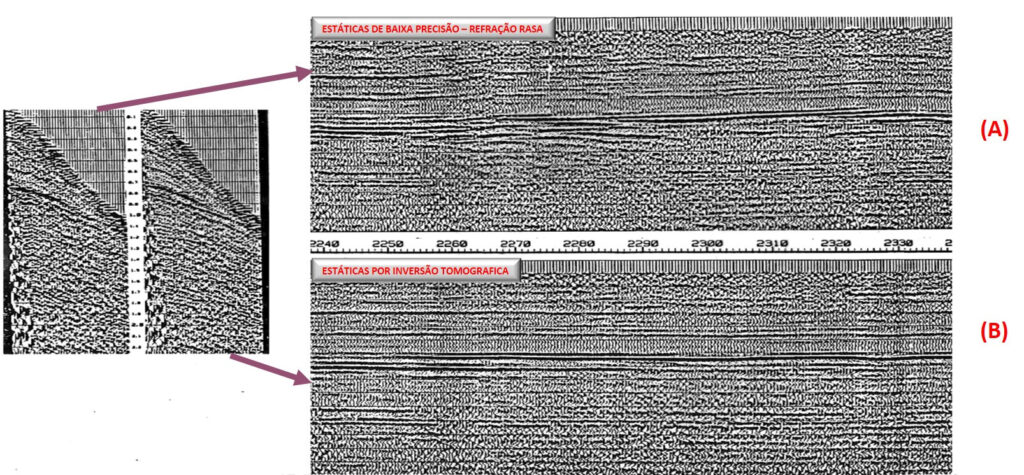
The figures below show the results obtained from processing a seismic line with low-precision static corrections (shallow refraction surveys) and the same line processed with static corrections calculated by tomographic inversion.
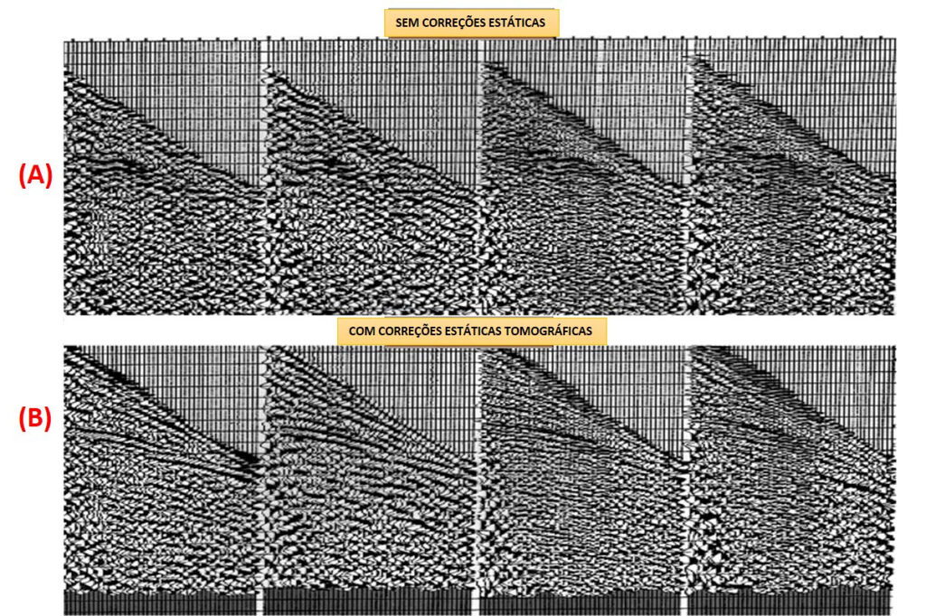
(A) WITHOUT STATIC CORRECTIONS (B) WITH STATIC CORRECTIONS. The figure above shows the result of the static corrections program of onshore seismic line field seismograms. Part (A) of the figure shows the seismograms without the static corrections program. Part (B) of the figure show the same seismograms with the static corrections calculated by tomographic inversion of the first breaks seismograms. Observe how the reflection hyperboles are well defined with the good precision static corrections shown in part (B) of the figure.
(A) LOW PRECISION STATIC (B) TOMOGRAPHIC INVERSION STATIC. The figure above shows the results of an onshore seismic line processing with good and bad quality static corrections. Part (A) of the figure shows the final seismic section with the application of low precision static corrections and part (B) of the figure shows the same line processed with tomographic inversion static correction calculations of the first break reflection seismograms. Observe that not only the image has better quality, but part (B) does not present long period static problems, which are responsible for structure formation and of short periods with loss in quality of stacking.
4– Enhancement of Low Frequency Software for Seismic Data
The spectrum of frequencies of a seismic signal has a limited band, for low as well as for high frequencies.
In conventional seismic surveys the sensors (geophones or hydrophones) cannot respond adequately to low frequencies (6 to 8 Hz). Thus, these elements should be prepared to deal with such signals, hence apart from introducing a significant phase distortion, the amplitudes are strongly attenuated. To obtain an acceptable register of the frequencies below these figures, it is necessary to utilize geophones similar to those used in seismology (earthquakes), which is not practical for seismic exploration surveys.
The low frequencies are strongly affected by superficial noise, very common in this frequency band. As such, the signal should be, and is registered in the field at a spectral band not contaminated by these effects.
Through the analysis of the seismic trace in the complex trace domain it is possible to extrapolate the frequencies outside of the useful frequency band of the original data. Via this analysis it is possible to obtain information relevant to the frequencies we want to stress and introduce them to the seismic data. With the frequencies calculated and inserted in each trace, their very own harmonics are found in the trace. To extrapolate the Low Frequencies, the pre-existing amplitude relations are not altered and have a small displacement from the signal phase.
This extrapolation can be used to better interpret the rock’s geometry, utilizing the low or high frequencies recovered for the original data.
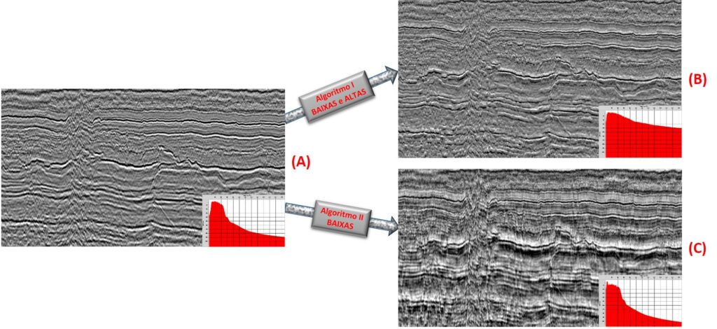
The figure above shows the result of the Enhancement of Low Frequency algorithm application on 2D onshore seismic data. Part (A) shows the line with conventional processing and its respective frequency spectrum. Part (B) shows the processing of section (A) using Enhancement of Low Frequencies using algorithm l. With this algorithm, not only does it enhance the Low Frequencies, but there is an extrapolation for the High Frequencies as well, as can be seen in the frequency spectrum. Part (C) shows the processing of section (A) using Enhancement of Low Frequencies using algorithm ll. This algorithm maintains the high frequency spectrum unaltered and extrapolates only for Low Frequencies. Note that with the Enhancement of Low Frequency there is a better definition of steep dip events, as expected. With this program there is a small displacement of the signal phase, but it possible to better separate the sedimentary packs.
5– Enhancement of High Frequency Software for Seismic Data
The spectrum of frequencies of a seismic signal has a limited band, for low as well as for high frequencies.
At high frequencies the limitation for registering the high frequencies is associated with the fact that sedimentary rocks have little elasticity and the seismic wave propagation provokes friction between adjacent grains and crystals and, quickly, the seismic energy is transformed into heat (absorption effect). This effect is greater as the vibrational frequencies get higher. If not for these limitations, we could register reflections with high resolution, showing the same information obtained in a sonic profile.
Through the analysis of the seismic trace in the complex trace domain it is possible to extrapolate the frequencies outside of the useful frequency band of the original data. Via this analysis it is possible to obtain information relevant to the frequencies we want to stress and introduce them to the seismic data. With the frequencies calculated and inserted in each trace, their very own harmonics are found in the trace. To extrapolate the High Frequencies, the pre-existing amplitude relations are not altered and there is no distortion in the signal phase and the reflector positions are preserved in their entirety. This attribute is reliable, only contains advantages and does not alter the seismic properties of the seismic section reflectors.
With the introduction of frequencies that richen the registered reflections, we create an attribute which enhances the seismographic packs and helps the correlation along the seismic section. The packs, or sequences, as they are defined, combine refection groups which have common characteristics, of the geological pack acoustic impedance.
This extrapolation can be used to help interpret the depositional systems, rock geometry and to better identify thinner layers.
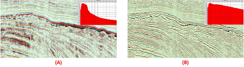
The figure above shows the result of the Enhancement of High Frequency algorithm application on 2D onshore seismic data. Part (A) shows the line with conventional processing and its respective frequency spectrum. Part (B) shows the processing of section (A) using Enhancement of High Frequencies. Observe that the frequency spectrum for the useful part of the original data remained unaltered, while at the top end of the spectrum there was great gain of the high frequency amplitudes. On part (B) of the figure we can observe that the wavelet was quite long, permitting more detailed studies of the geometrical relations between the diverse strata. There is no loss of events and perfect conservation of reflector positioning.
6– Kirchhoff Pre-Stacking Migration of Floating Datum and Final Datum Software.
Reflection seismic data pre-stack migration programs, whether for 2D or 3D data, are generally designed for application to seismic data in the Final Surface Datum. However, stacking velocities are calculated using data in the Floating Datum, and for migration to be performed, an adjustment in these velocities is required. Often, these velocities differ significantly from stacking velocities, depending on the distance between the Floating Datum and the Final Surface Datum. That is, the greater this distance, the greater the difference between the velocities, making it more challenging to adjust the reflection curves by hyperbolic curves assumed in the data migration process. This affects the quality of the final migrated sections.
Thus, it becomes necessary to have programs capable of performing pre-stack migration in the Floating Datum and also have the option to migrate in the Final Surface Datum, for cases of small separation between the two datums.
The company CImaGeo has developed its own migration program based on articles published in the geophysical literature and utilizing parts of source codes available in libraries open to the worldwide geophysical community. It takes into account all necessary amplitude corrections for performing time migrations.
Tests conducted with synthetic and real data, both for straight lines and "crooked" geometry, show that the results are of high quality, and the reliability regarding phase and amplitudes is quite high.
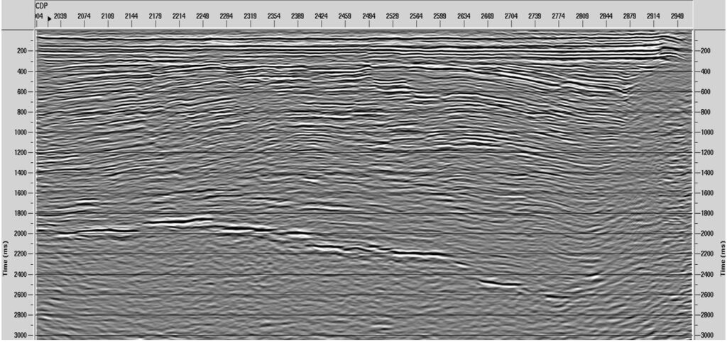
The figure above shows a land seismic section with pre-stack time migration (Kirchhoff) performed on the floating datum. In many situations, the final datum is far from the floating datum, and it becomes necessary to perform migration on the floating datum, where velocities are more consistent with the seismic data. After migration, the program itself takes the section to the final flat datum.
7– Speed Analysis Software using CVS
The velocity analysis stage, for stacking or migration, is one of the critical points in reflection seismic processing, and its effectiveness and accuracy will determine the quality of data stacking.
Generally, processing packages offer velocity analysis programs in which analysis points (CDPs) are chosen a priori by the geophysicist, and velocity panels are calculated only in the vicinity of those points. Therefore, there is a restriction on densifying the analyses in regions where geology is more complex and the distance between analyzed points should be smaller.
The company CImaGeo has developed a velocity analysis program that utilizes the CVS (Constant Velocity Stack) philosophy, in which the entire seismic section is stacked multiple times, each with a constant velocity, with velocity increment defined by the geophysicist. From these panels, velocity analysis can be performed at any point (CDP) of the seismic section, aided by the supergather and semblance function at that point.
This approach enables velocity analysis at any point of the seismic section, with denser point spacing in areas where geology is more complex, either due to structural reasons or lateral velocity variations.
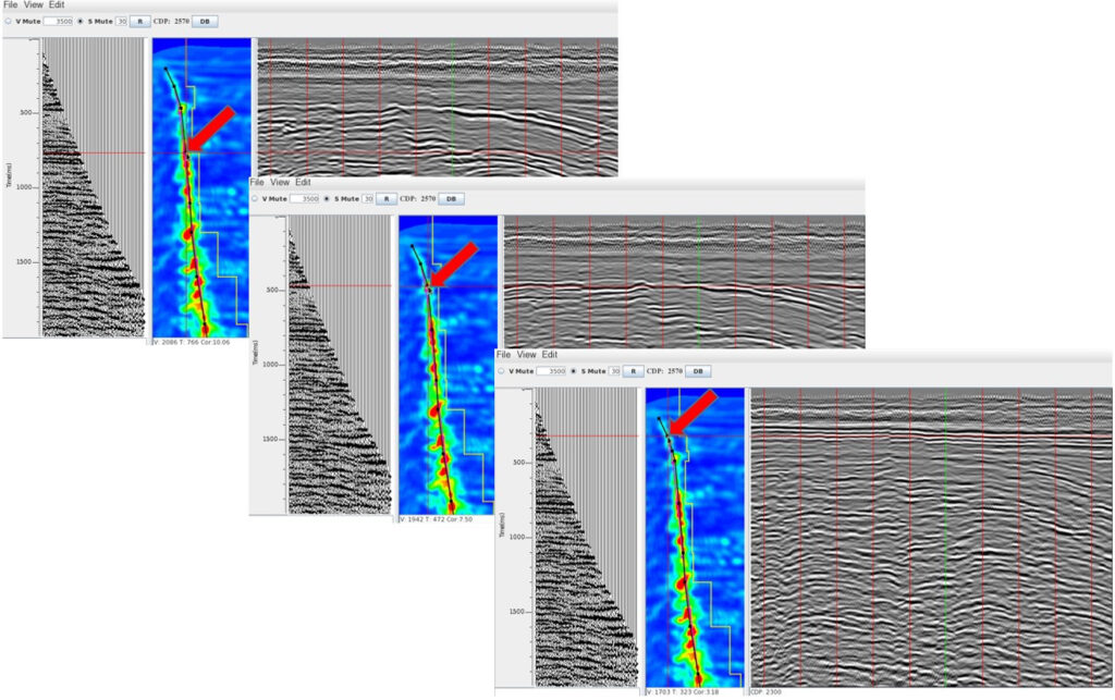
The figure above shows three velocity analysis panels of a seismic line. Each panel consists of a supergather (left), semblance function (center), and the stacked seismic section with velocity indicated by the mouse position on the semblance (red arrow). Each vertical line in the seismic section indicates a point where velocity analysis was performed, with the current point highlighted in green. The geophysicist positions the mouse at any point along the line where velocity analysis is desired, and can densify the points as needed. The seismic section is stacked multiple times with constant velocity at intervals defined by the geophysicist.
8–Mute Analysis Software using CVS
During the process of applying NMO (Normal Move Out) correction, signals undergo stretching inherent to the process, which must be avoided in the stacking process to prevent degradation of stacking quality due to distortion in the recorded wavelet.
In general, the elimination of these stretched data is carried out through automatic processes, where the geophysicist specifies the maximum percentage of wavelet stretching that will be allowed, and any data with greater distortion is removed in a process called mute or silencing. Another way is through visual analysis of NMO-corrected CDPs, where the geophysicist defines the range of offsets for which the data will be used and eliminates the rest.
Another common method in processing packages is partial stacking with increasing offsets, using small segments around the chosen analysis points (CDPs). In this way, since the points are chosen, there is a difficulty in densifying in areas of more complex geology.
The company CImaGeo has developed a mute analysis program in which the entire seismic section is stacked with the last velocity analysis in a process of partial stacking, where the first section is stacked with short offsets and additional offsets are added for subsequent sections in bands predefined by the geophysicist. This way, during the interpretation process, the geophysicist can densify points in areas where the geology becomes more structurally complex or where there are more abrupt lateral variations.
This process can be iteratively repeated with previous analyses for result refinement.
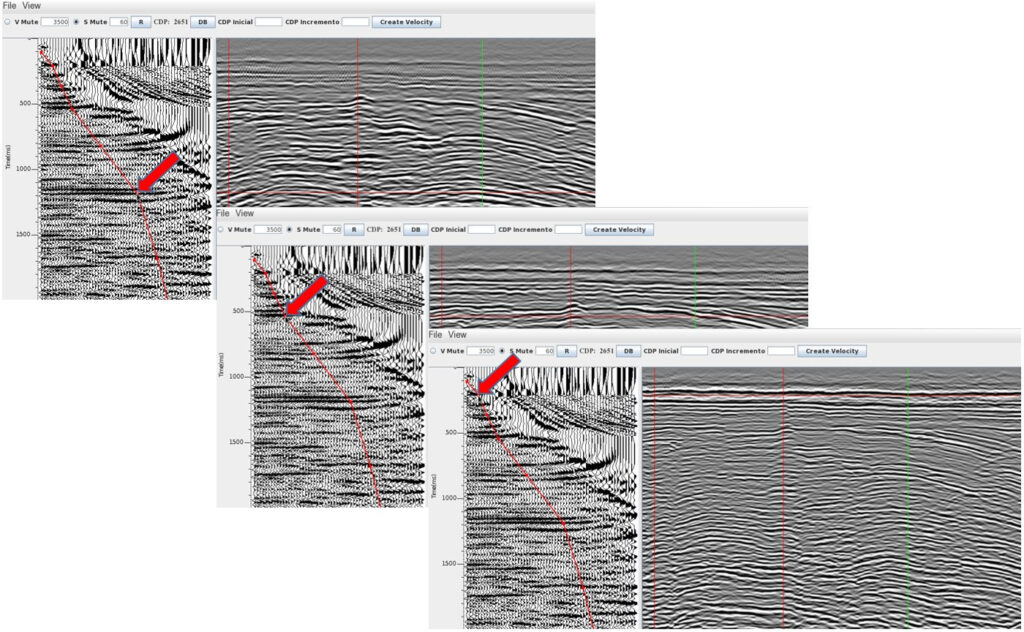
The figure above shows three mute analysis panels of a seismic line. On the left side of the panel, the corrected NMO (normal moveout) CDP (common depth point) is displayed without any mute, while on the right side, the stacked seismic section with a set of distinct offsets ("partial stacks") is shown. It starts with the shortest offsets, and for each new section, additional offsets (increasing) are added in steps defined by the geophysicist. Each vertical line in the seismic section indicates a point where mute analysis was performed, with the current point highlighted in green. The geophysicist positions the mouse at any point along the line where mute analysis is desired, and on the CDP, they choose the section to be displayed on the screen, corresponding to the stacking of that set of offsets, which will show the effect of stretched data entry on stacking. The geophysicist can densify the analysis points as much as necessary.
9- Geometry and Elevation Quality Control Software using NASA’s WorldWind.
After defining the geometry of the seismic data using field files and the Observer Report, a plot of the line is made on the NASA WorldWind satellite image. The elevation from this image is then extracted and visually compared with the field topography of the line being processed.
Although the accuracy of the topography from satellite images may not be suitable for use as the elevation of the line, it is used to verify its positioning. This is because in many cases of old lines, there may be conflicting or even missing topographic information. In such cases, the satellite elevation will need to be used for processing that line, or the line will not be processed and will be lost.
At times, it is possible to identify missing data in certain sections of the seismic line simply by visualizing the line's drawing on the satellite image. The geophysicist should then investigate what may have occurred and rectify the error.
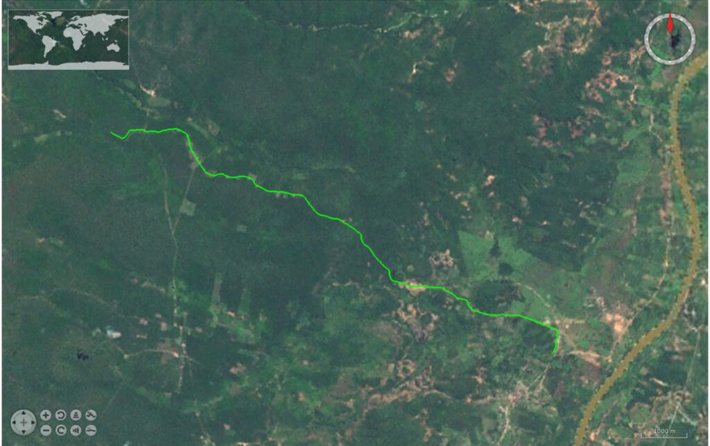
The figure above shows a seismic line plotted on a NASA WorldWind satellite image. In cases where there is an issue with the geometry of the line, this image allows for locating points for subsequent correction. It can also be used to verify positioning errors. For example, in the case above, there is a crooked line that should be over a road, and this information can be confirmed in the image. Additionally, a topographic profile can be generated to be compared with the field survey profile.
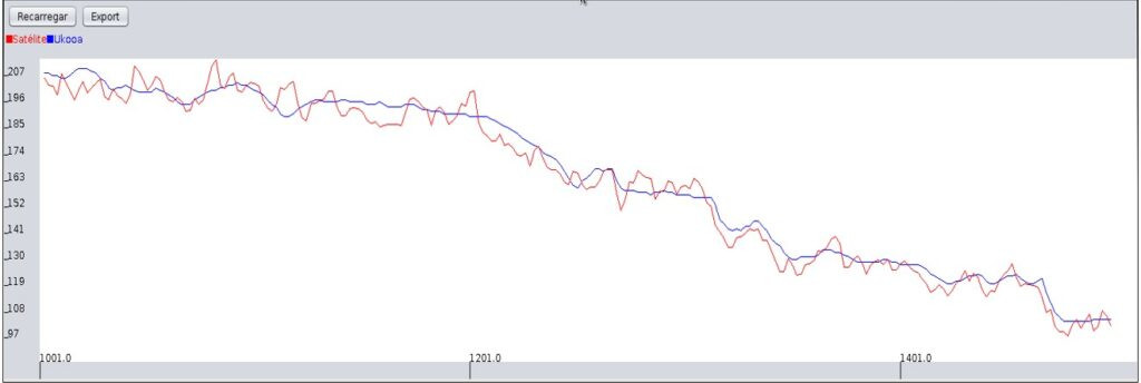
The figure above shows the topographic profile of the seismic line with field measurements (red) and the same profile recovered from the NASA WorldWind satellite image (blue). Note that the topography recovered from the image lacks the necessary precision for its use as the line's topography. However, it can be used to verify positioning and also indicate points in the topography that need to be checked.
10– Software developed for ProMax/SeisSpace.
For optimal utilization of the software's entire computational infrastructure and to avoid importing SeisSpace (ProMax / JavaSeis) and exporting data to its structure, whenever possible, the applications developed at CImaGeo are integrated into the computational framework of SeisSpace (ProMax / JavaSeis), this results in better computational performance and time savings in seismic data processing.